You may need more time if programming is completely new to you, or less if you have some experience already.
Instructions
The quiz is closed book/note/computer/phone
If you need to use the restroom, leave your exam and phone with the TA
You have 60 minutes to complete the quiz. If you finish early, you may turn in your quiz and leave early
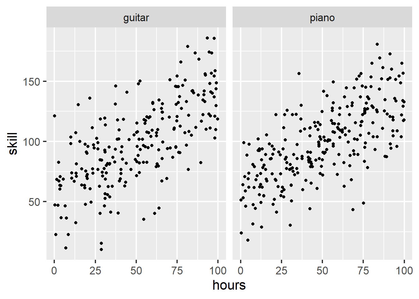
The data
Suppose we want to study the effect hours practicing an instrument has on your ultimate skill level with the instrument. We study 500 participants who are learning to play either piano or guitar. Below we explore these data in a few ways.
Suppose we fit a model represented by the following equation, where \(x_1\) is the number of hours spent practicing, \(x_2\) is the instrument, and \(y\) is the skill acheived:
\(y = b_0 + b_1x_1 + b_2x_2\)
Which of the following would work to estimate the free parameters of this model? Choose one.
only gradient descent
only ordinary least squares
both gradient descent and ordinary least squares
True or false, when performing gradient descent on a nonlinear model, we might arrive at a local minimum and miss the global one.
True
False
True or False, given the model above, gradient descent and ordinary least squares would both converge on approximately the same parameter estimates.
True
False
The following plots a linear model of the formula y ~ 1 + x and one data point. Which dashed line represents the model’s residual for this point? Circle one.
Which of the following could be the model specification in R? Choose all the apply.
skill ~ hours + instrument_recoded
skill ~ hours * instrument_recoded
skill ~ 1 + hours + instrument_recoded
In the code, SSE() is a function we have defined to calculate the sum of squared errors. Which of the following correctly describes the steps of calculating SSE? Choose one.
1) calculate the residuals, 2) square each of the residuals, 3) add them up
1) calculate the residuals, 2) add them up, 3) square the sum of residuals
1) calculate the residuals, 2) calculate their standard deviation, 3) square it
1) calculate the residuals, 2) calculate their mean, 3) square it
Using the estimated parameters from lm(), fill in the blanks to calculate the model’s predicted value of skill for a participant who played the piano for 20 hours. You may round to the first decimal place.
skill = 58.9 + ( 0.8 * 20 ) + ( 0.7 * 1 )
Which of the following is the most likely value of the sum of squared errors when the parameters \(b_0\), \(b_1\), and \(b_2\) are all set to 0? Choose one.
exactly 0
exactly 286497.6
a value higher than 286497.6
a value lower than 286497.6
3 Model Accuracy
Questions in section 3 refer to the following summary() of the same model from section 2:
Which of the following is a correct interpretation of the model’s \(R^2\) value? Choose one.
The model has a 46.49% chance of explaining the true pattern in the data.
The model explains 46.49% of the variance found in the data.
The sample shows 46.49% of the variance found in the population.
Which of the following is true about the model’s \(R^2\)? Choose all that apply.
tends to overestimate \(R^2\) on the population
tends to underestimate \(R^2\) on the population
tends to overestimate \(R^2\) on the sample
tends to underestimate \(R^2\) on the sample
Which one of the following is true about \(R^2\)? Use the below formula as a guide and choose one.