# load the packages we needlibrary(tidyverse)library(infer)# set the theme of all figurestheme_set(theme_classic(base_size =14))# set a seed so we get the same random stuff every timeset.seed(60)# generate some data for female penn studentsfemales <-tibble(volume =rnorm(5625, mean =1200, sd =92),sex ="female")# generate some data for male penn studentsmales <-tibble(volume =rnorm(5625, mean =1220, sd =98),sex ="male")# make the whole population penn_pop <-bind_rows(males, females)# sample 200 participants from this populationpenn_sample <- penn_pop %>%slice_sample(n =200)# get just the female and just the male participants# to use in figures penn_sample_f <-filter(penn_sample, sex =="female")penn_sample_m <-filter(penn_sample, sex =="male")# compute the mean to use in some figures mean_f <-mean(penn_sample_f$volume)mean_m <-mean(penn_sample_m$volume)
Last week we explored a simple dataset in which we measured brain volume for a sample of Penn students and computed the mean. Suppose we now want to take into account the sex of the students. What can we do with these data?
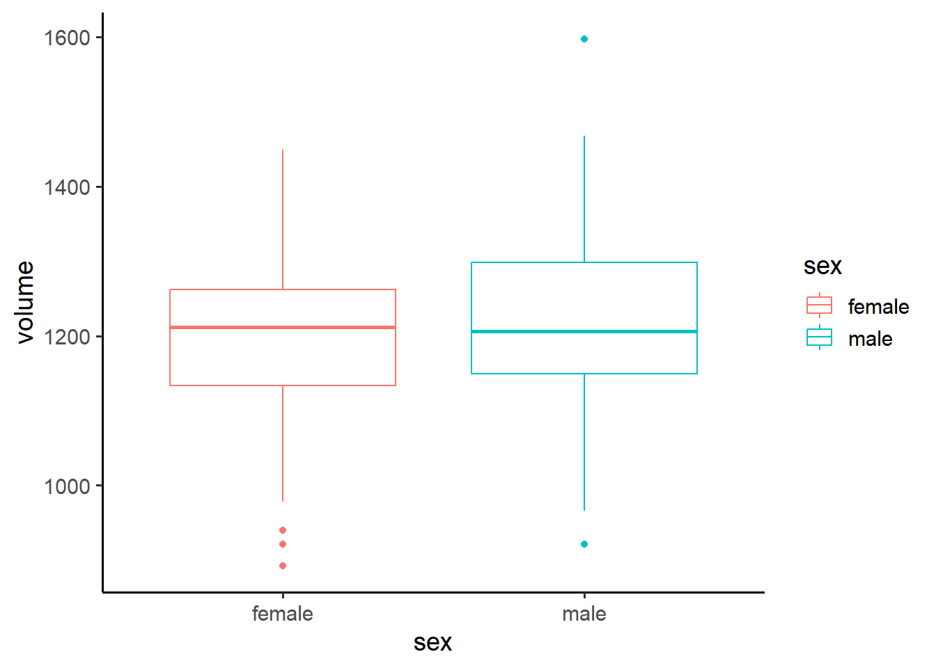
The first thing we should do is visualize our data. A useful visualization for a categorical variable is a boxplot:
penn_sample %>%ggplot(aes(y = volume, x = sex)) +geom_boxplot(aes(color = sex))
One thing we might want to ask is whether the two sexes differ in mean brain volume. Let’s compute the difference we observe in our sample with infer:
obs_diff <- penn_sample %>%specify(response = volume, explanatory = sex) %>%calculate(stat ="diff in means", order =c("male", "female"))obs_diff
Response: volume (numeric)
Explanatory: sex (factor)
# A tibble: 1 × 1
   stat
  <dbl>
1  19.2
Last week we saw that the mean of any sample drawn from the population will be subject to sampling variability. The same situation applies here: the difference in means will also differ depending on our sample. Thus, even if we find a difference in means, that difference could be due to sampling error (not any true difference in the population).
1 Hypothesis testing framework
To determine whether the brains of male and female Penn students differ with respect to the mean, we can use a framework for decision making called hypothesis testing. We can think of this as a 3-step process:
First we pose a null hypothesis that our result is due to nothing but chance (sampling variability)
Then we ask: if the null hypothesis is true, how likely is our observed pattern of results? This liklihood is the p-value.
Finally, if the p-value is less some threshold we decide upon (<0.05) then we reject the null hypothesis.
1.1 Step 1: Pose the null hypothesis
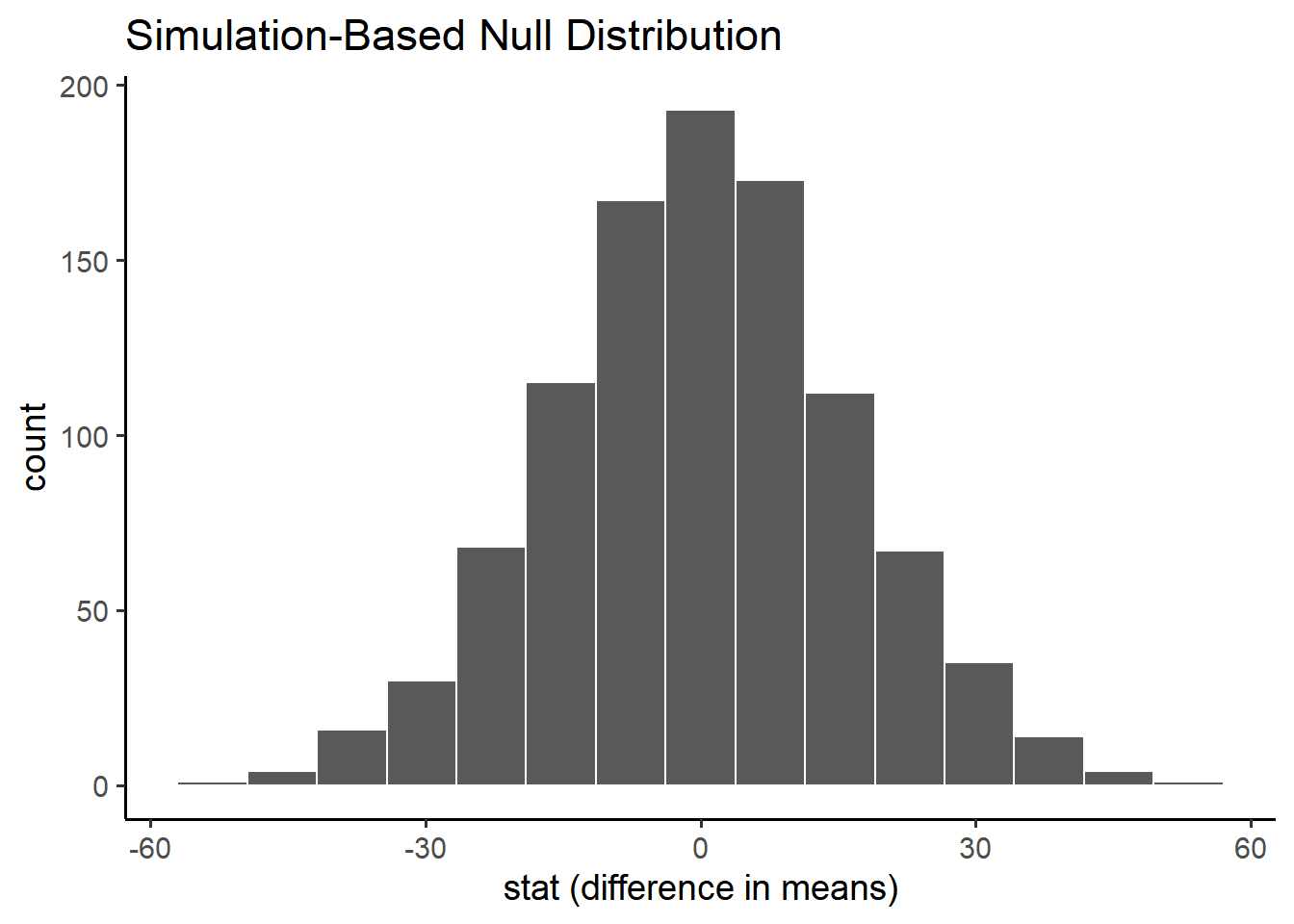
We pose a null hypothesis for practical reasons: it is the hypothesis for which we can simulate data. We can construct the sampling distribution for a hypothetical world in which our observed value is due to chance (we call this the null distribution).
To construct the null distribution we can use a process called randomization.
Randomization is similar to bootstrapping except, on each repeat, we will shuffle the sex and randomly assigning it to each participant.
This simulates a world in which there is no relationship between brain volume and sex.
Show code
null_distribution <- penn_sample %>%specify(response = volume, explanatory = sex) %>%hypothesize(null ="independence") %>%generate(reps =1000, type ="permute") %>%calculate(stat ="diff in means", order =c("male", "female")) null_distribution %>%visualize() +labs(x ="stat (difference in means)")
1.2 Step 2: How likely is our observed pattern?
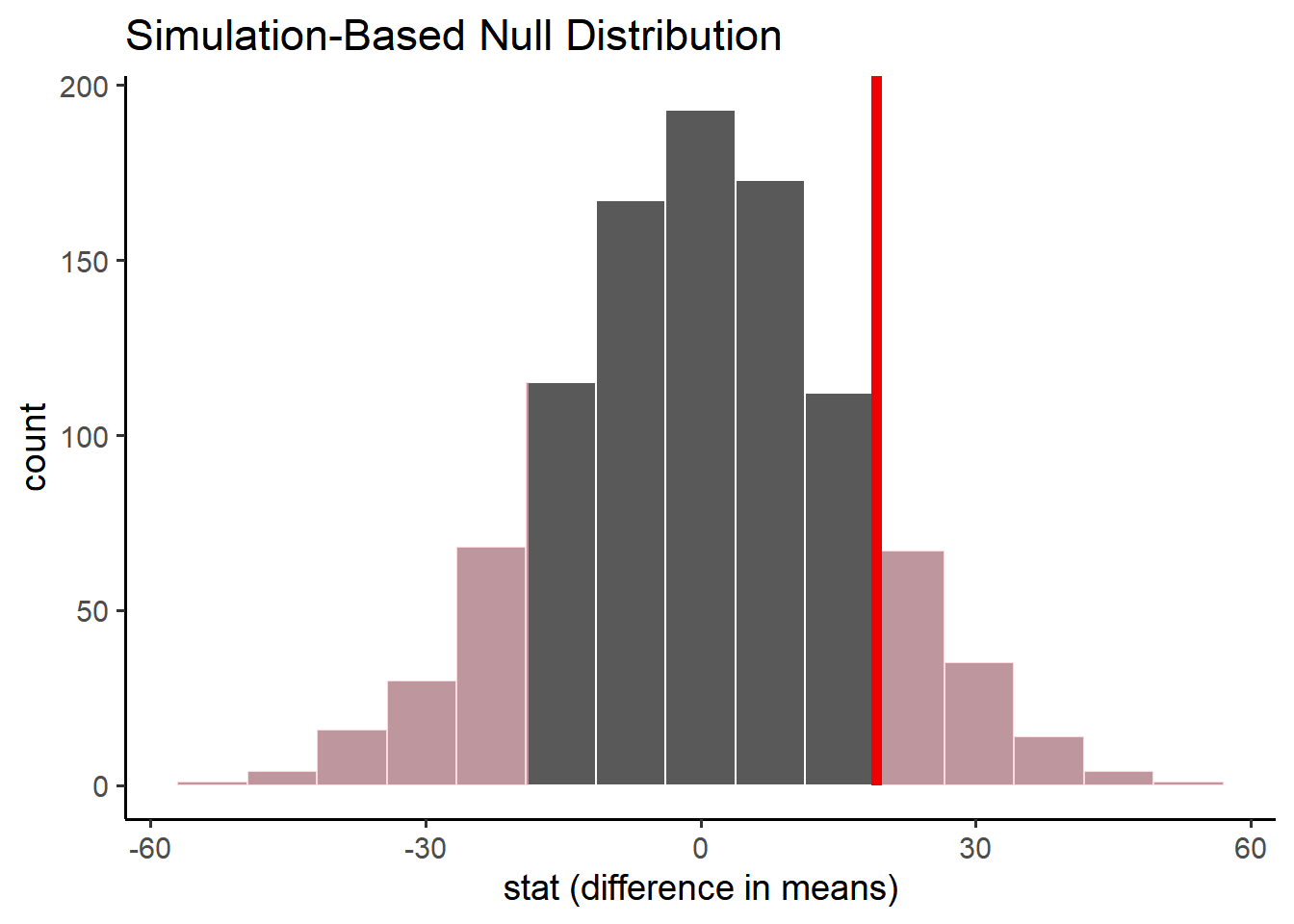
If the null hypothesis is true, how likely is our observed pattern of results? We can quantify this liklihood directly with the p-value: count the number of values in our null distribution that are more extreme than our observed value and divide that by the number of simulations we generated.
Or infer can handle this for us with the get_p_value() function:
null_distribution %>%get_p_value(obs_stat = obs_diff, direction ="both")
# A tibble: 1 × 1
  p_value
    <dbl>
1   0.242
A large p-value means our observed value is very likely under the null hypotheisis. A small p-value means our observed value is very unlikely under the null hypothsis.
Show code
obs_diff <- penn_sample %>%observe( volume ~ sex,stat ="diff in means",order =c("male", "female") )null_distribution %>%visualize() +shade_p_value(obs_stat = obs_diff, direction ="two-sided") +labs(x ="stat (difference in means)")
Warning in (function (mapping = NULL, data = NULL, stat = "identity", position = "identity", : All aesthetics have length 1, but the data has 1000 rows.
ℹ Did you mean to use `annotate()`?
1.3 Step 3: Decide whether to reject the null
Finally, if the p-value is small enough — less than some threshold we decide upon — we reject the null hypothesis. By convention we consider a p-value less than 0.05 to be implausible enough that we can reject the null hypothesis (read more about why 0.05. Note that obtaining our observed value is implausible under the null, but not impossible. In other words, our decision to reject (or not) could be wrong!
When we reject a null hypothesis that was actually true, we call it a type I error.
When we fail to reject a null hypothesis that was actually false, we call it a type II error
This figure borrowed from reddit can help you remember the error types. (Null hypothesis here is “NOT pregnant”)
Do you know the “The boy who cried wolf” story?
Remembering which error is I or II can be tricky. June likes to analogize it to “The boy who cried wolf” to remember errors in chronological order:
Type I error is the first thing that happens: Townspeople think there is a wolf, but it’s not actually there! (false positive - wrongly thinking that the effect is present)
Type II error is the second thing that happens: The wolf actually appears but townspeople don’t believe it! (false negative - wrongly thinking that the effect is absent)
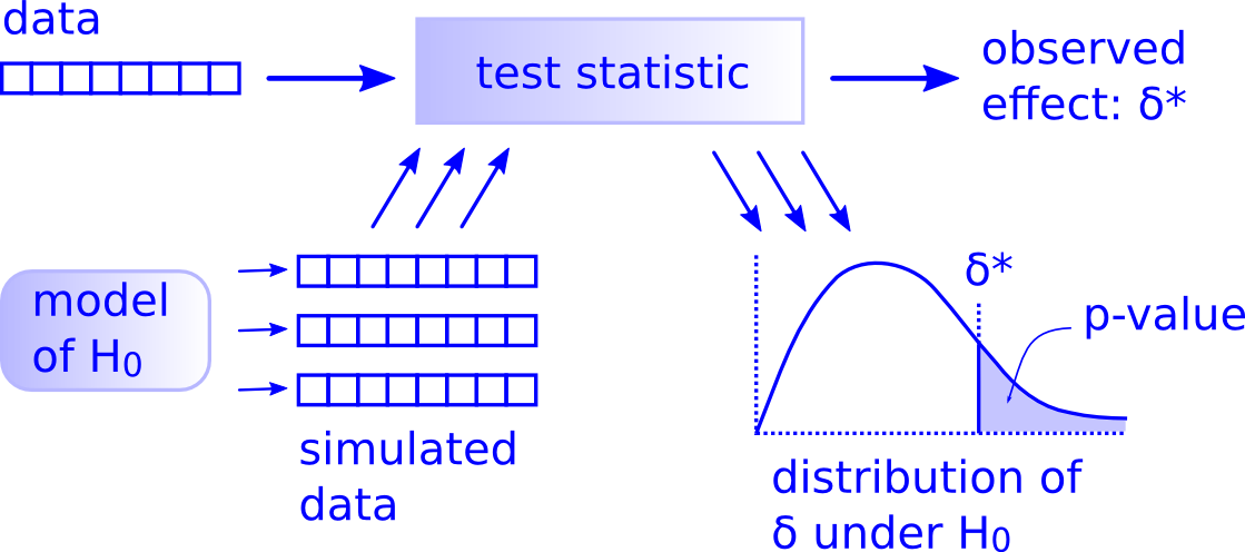
2 There is only one test
Figure borrowed from Modern Dive textbook
Computer scientist Allen Downey famously dubbed the framework outlined above the “There is only one test” framework. It allows us to appreciate that, though there are a myriad of statistical tests available, there is really only one hypothesis test. If you understand this general framework, you can understand any hypothesis test (t-test, chi-squared, etc).
Remember from last week that there are two ways we can construct a sampling distribution (simulate data):
Nonparametrically, via brute computational force (simulating many repeats of the same experiment with bootstrapping or randomization)
Parametrically, by assuming the data were sampled from known probability distribution and working out what happens theoretically under that distribution.
In the approach above, I’ve demonstrated the nonparametric way. But we could have opted for a parametric test instead. Let’s illustrate with a t-test.
2.1 t-test example
We can use R’s built in function to perform a t-test to compare two means.
    Welch Two Sample t-test

data:  penn_sample_m$volume and penn_sample_f$volume
t = 1.1921, df = 197.16, p-value = 0.2347
alternative hypothesis: true difference in means is not equal to 0
95 percent confidence interval:
 -12.56993  50.99280
sample estimates:
mean of x mean of y
 1220.573  1201.362
Under the hood, the t.test() is performing the same “one test”, it is just constructing the null distribution parametrically (assuming a known probability distribution defined by parameters). We can see this with infer by asking it to assume() a distribution rather than generate() data.
# calculate the observed value (t)obs_val <- penn_sample %>%specify(response = volume, explanatory = sex) %>%calculate(stat ="t",order =c("male", "female")) obs_val
Response: volume (numeric)
Explanatory: sex (factor)
# A tibble: 1 × 1
   stat
  <dbl>
1  1.19
# assume the t distribution null_distribution_theo <- penn_sample %>%specify(response = volume, explanatory = sex) %>%assume(distribution ="t") # return the p value null_distribution_theo %>%get_p_value(obs_val, direction ="both")
# A tibble: 1 × 1
  p_value
    <dbl>
1   0.235
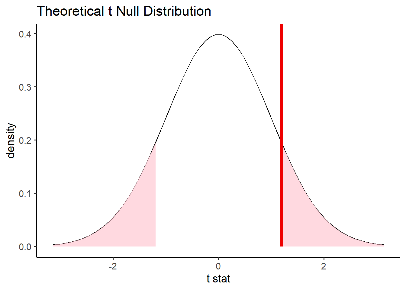
# visualize the theoretical distributionnull_distribution_theo %>%visualize() +shade_p_value(obs_val, direction ="both")
3 Exploring relationships
So far we explored data in which we measured a single quantity: brain volume. Suppose we have a slightly more complex dataset in which we measure two quantities! Let’s use the ratings data from the languageR package.
library(languageR)
We might want to know whether there is a relationship between two variables. We can explore the relationship between two quantities visually with a scatter plot.
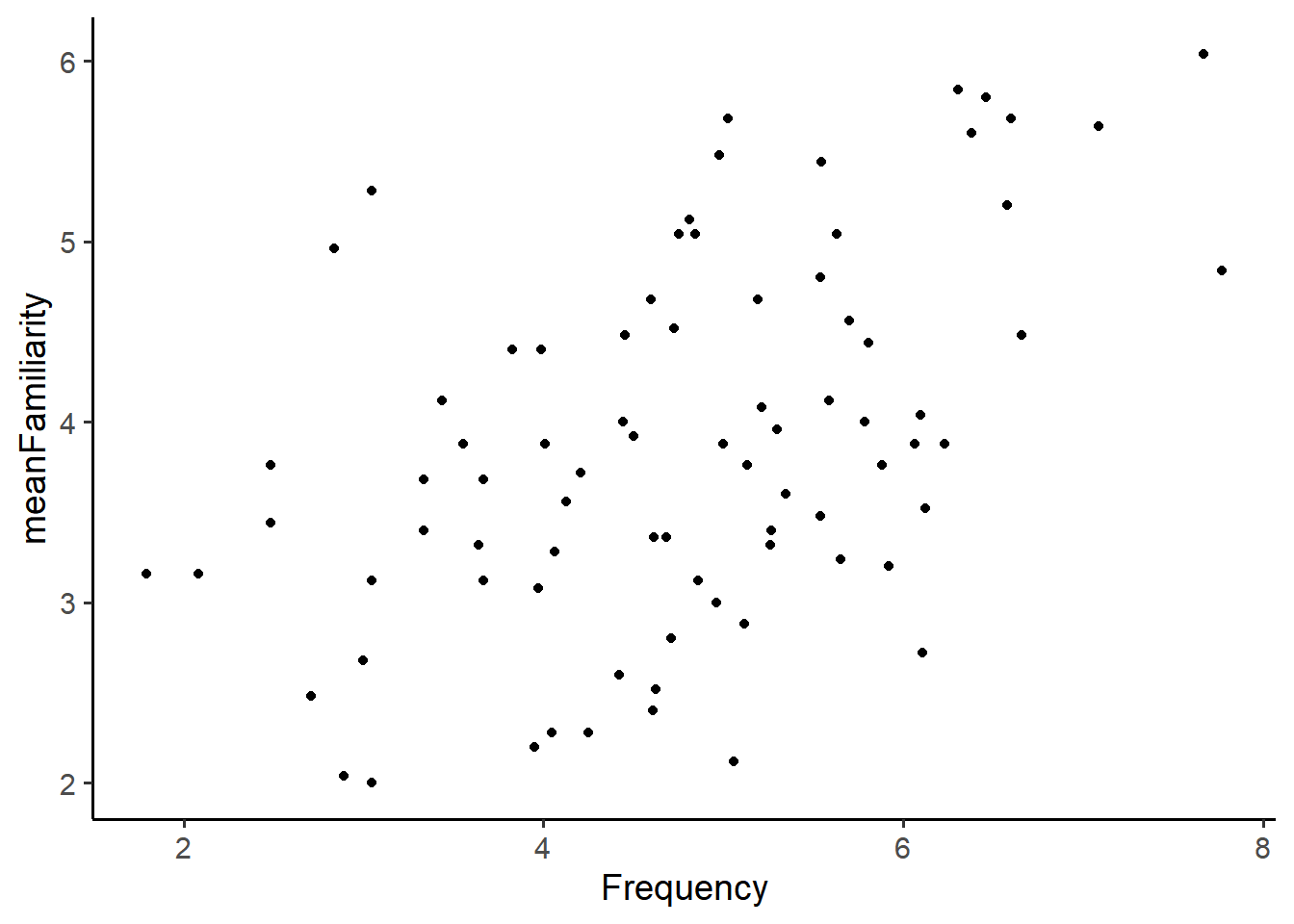
ratings %>%ggplot(aes(x = Frequency, y = meanFamiliarity)) +geom_point()
If there is no relationship between the variables, we say they are independent. We can think of independence in the following way: knowing the value of one variable provides no information about the other variable. In the ratings data, that would mean the word’s actual frequency provides provides no information about the participants mean familiarity rating. If there is some relationship between the variables, we can consider two types:
There may be a linear relationship between the variables. When one goes up the other goes up (positive) or when one goes up the other goes down (negative). In our example, there is a linear relationship between meanFamiliairity and Frequency: as Frequency increases, meanFamiliarity also increases.
Or a nonlinear relationship. Nonlinear is a very broad category that encompasses all relationships that are not linear (e.g. a U-shaped curve).
4 Correlation
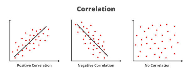
One way to quantify linear relationships is with correlation (\(r\)). Correlation expresses the linear relationship as a range from -1 to 1, where -1 means the relationship is perfectly negative and 1 means the relationship is perfectly positive.
Figure borrowed from iStock photos
Correlation can be calculated by taking the z-score of each variable (a normalization technique in which we subtract the mean and divide by the standard deviation) and then computing the average product of each variable:
Or we can use R’s built in correlation function: cor(x,y)
cor(ratings$Frequency, ratings$meanFamiliarity)
[1] 0.4820286
Just like the mean — and all other test statistics! — \(r\) is subject to sampling variability. We can indicate our uncertainty around the correlation we observe in the same way we did for the mean last week: construct the sampling distribution of the correlation via bootstrapping and compute a confidence interval.
# get the observed correlation obs_corr <- ratings %>%specify(response = meanFamiliarity, explanatory = Frequency) %>%calculate(stat ="correlation")obs_corr
Response: meanFamiliarity (numeric)
Explanatory: Frequency (numeric)
# A tibble: 1 × 1
   stat
  <dbl>
1 0.482
# construct the sampling distributionsamp_dist <- ratings %>%specify(response = meanFamiliarity, explanatory = Frequency) %>%generate(reps =1000, type ="bootstrap") %>%calculate(stat ="correlation")
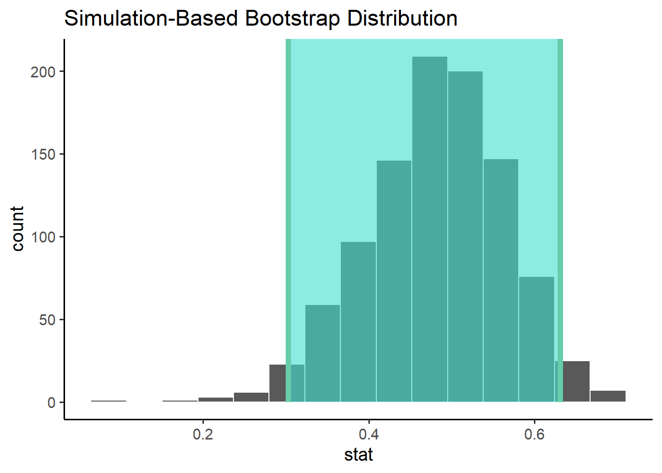
# compute a confidence intervalci <- samp_dist %>%get_confidence_interval(level =0.95, type ="percentile")ci
# visualize the distribution samp_dist %>%visualize() +shade_ci(ci)
How do we test whether the correlation we observed in the data is significantly different from zero? We can use hypothesis testing (as learned today)! Here our null hypothesis that there is no relationship between the variables (they are independent). First we generate the null distribution:
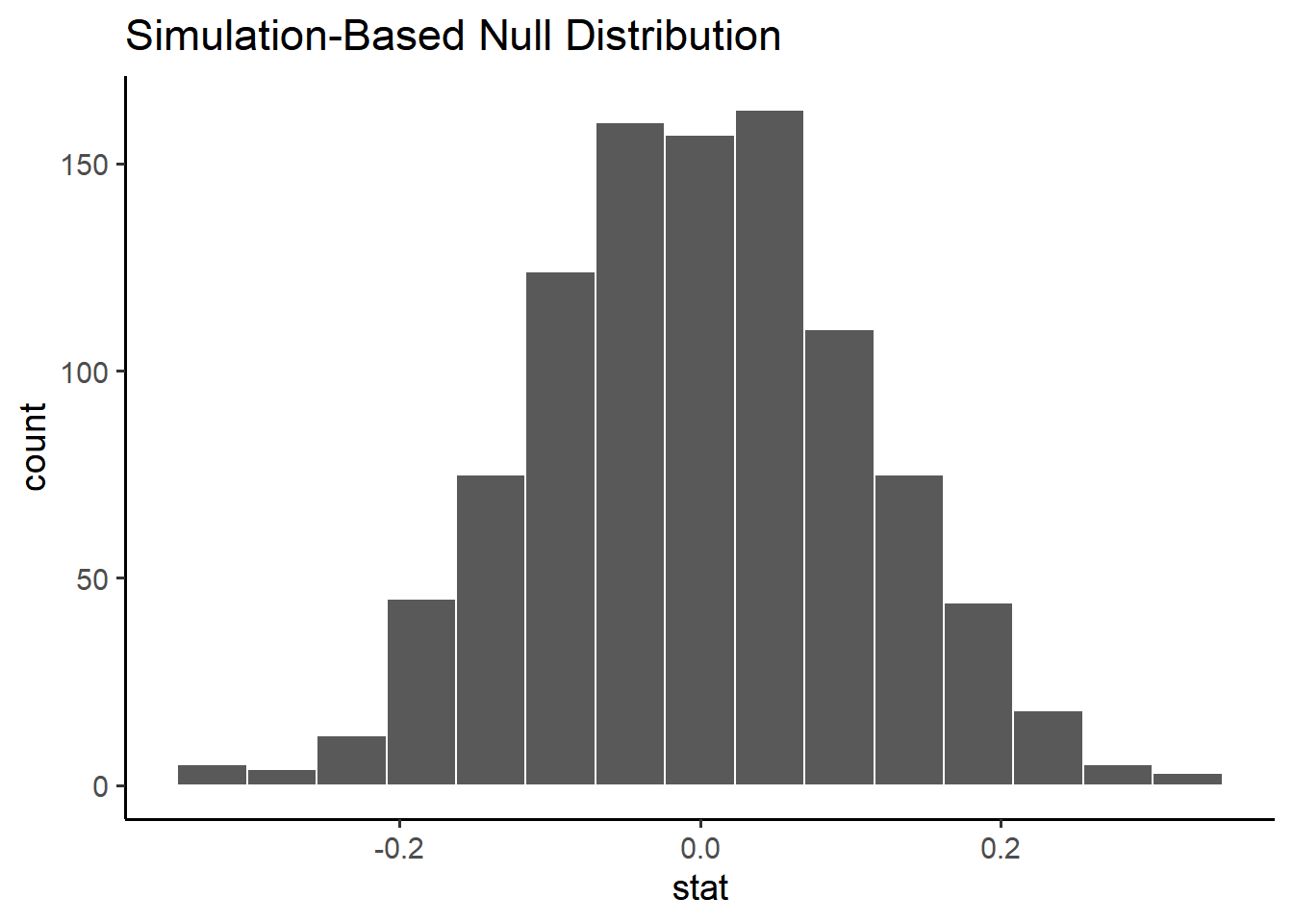
# generate the null distribution null_distribution_corr <- ratings %>%specify(response = meanFamiliarity, explanatory = Frequency) %>%hypothesize(null ="independence") %>%generate(reps =1000, type ="permute") %>%calculate(stat ="correlation") null_distribution_corr %>%visualize()
Then we ask how likily our observed correlation is under the null hypothesis (get a p-value):
# get the p-valuenull_distribution_corr %>%get_p_value(obs_stat = obs_corr, direction ="both")
Warning: Please be cautious in reporting a p-value of 0. This result is an
approximation based on the number of `reps` chosen in the `generate()` step.
See `?get_p_value()` for more information.
# A tibble: 1 × 1
  p_value
    <dbl>
1       0
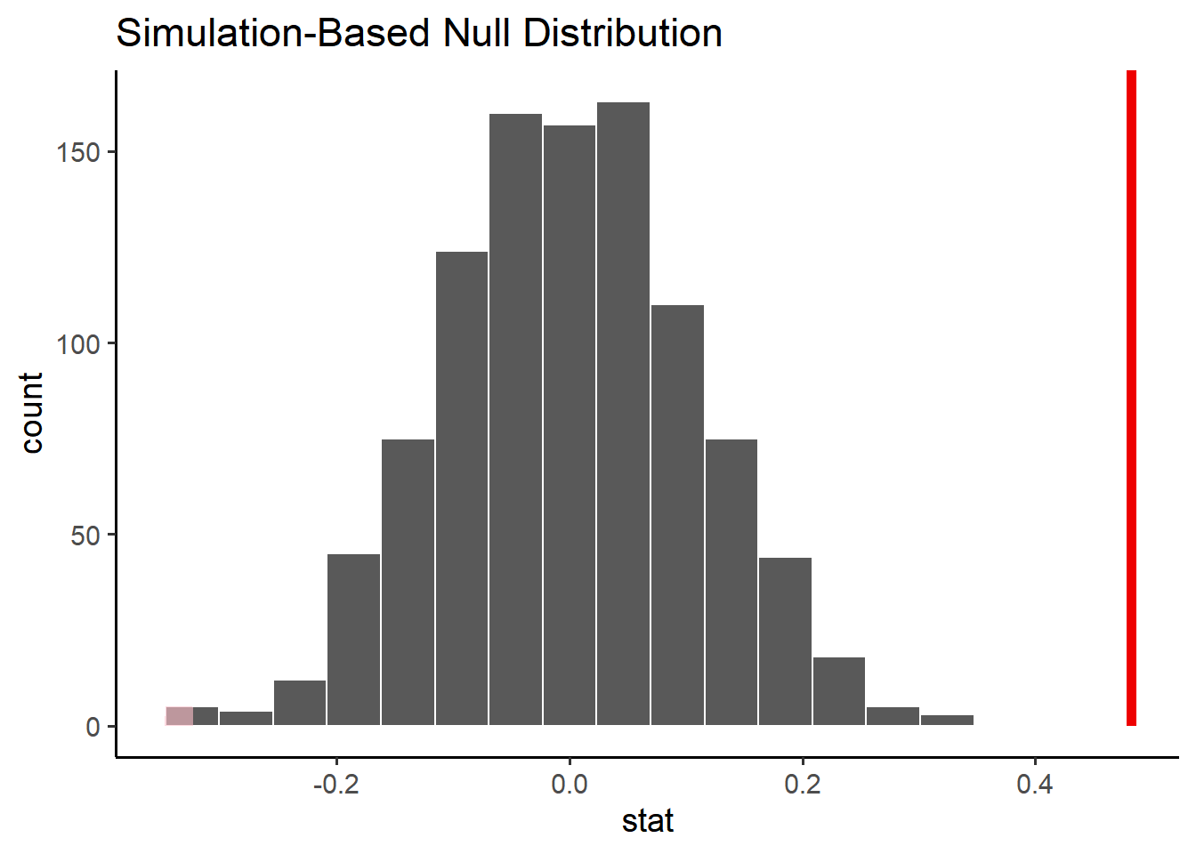
# visualize p-value on the null distributionnull_distribution_corr %>%visualize() +shade_p_value(obs_stat = obs_corr, direction ="two-sided")
Warning in (function (mapping = NULL, data = NULL, stat = "identity", position = "identity", : All aesthetics have length 1, but the data has 1000 rows.
ℹ Did you mean to use `annotate()`?
Finally we decide whether to reject the null hypothesis if the liklihood of observing this correlation under the null is small enough (<0.05). We can see that our observed correlation is very unlikely in the null distribution (p-value = 0), so we reject the null hypothesis.