# A tibble: 10 × 1
   volume
    <dbl>
 1  1193.
 2  1150.
 3  1243.
 4  1207.
 5  1236.
 6  1292.
 7  1201.
 8  1259.
 9  1157.
10  1169.
Rows: 5,216
Columns: 1
$ volume <dbl> 1193.283, 1150.383, 1242.702, 1206.808, 1235.955, 1292.399, 120…Data Science for Studying Language and the Mind
2024-09-17
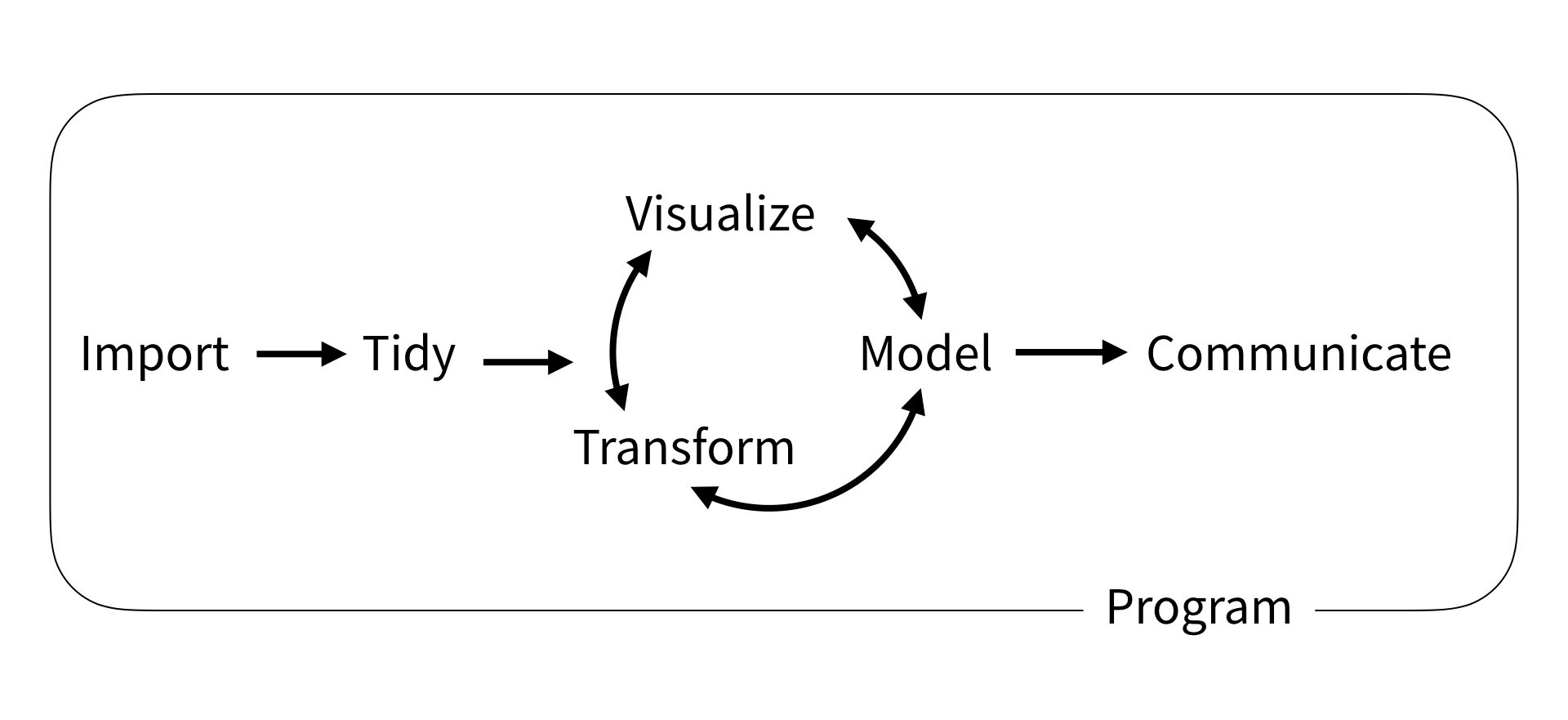
Data Science Workflow by R4DS
Each tick mark is one data point: one participant’s brain volume
Visualize the distribution of the data with a histogram
Summarize the data with a single value: mean, a measure of where a central or typical value might fall

Summarize the data with a single value: mean, a measure of where a central or typical value might fall
Summarize the spread of the data with standard deviation
Summarize the spread of the data with standard deviation

Suppose we have a non-normal distribution

mean() and sd() are not a good summary of central tendency and variability anymore.
Instead we can use the median as our measure of central tendency: the value below which 50% of the data points fall.
And the interquartile range (IQR) as a measure of the spread in our data: the difference between the 25th and 75th percentiles (50% of the data fall between these values)

We can calculate any arbitrary coverage interval. In the sciences we often use the 95% coverage interval — the difference between the 2.5 percentile and the 97.5 percentile — including all but 5% of the data.

All possible values are equally likely
The probability density function for the uniform distribution is given by this equation (with two parameters: min and max).
One of the most useful probability distributions for our purposes is the Gaussian (or Normal) distribution
The probability density function for the Gaussian distribution is given by the following equation, with the parameters \(\mu\) (mean) and \(\sigma\) (standard deviation).
When measuring some quantity, we are usually interested in knowning something about the population: the mean brain volume of Penn undergrads (the parameter)
But we only have a small sample of the population: maybe we can measure the brain volume of 100 students
Any statistic we compute from a random sample we’ve collected (parameter estimate) will be subject to sampling variability and will differ from that statistics computed on the entire population (parameter)
If we took another sample of 100 students, our parameter estimate would be different.
The sampling distribution is the probability distribution of values our parameter estimate can take on. Constructed by taking a random sample, computing stat of interest, and repeating many times.
Our first sample was on the low end of possible mean brain volume.
Our second sample was on the high end of possible mean brain volume.
The spread of the sampling distribution indicates how the parameter estimate will vary from different random samples.
parametric statistic because we assume a gaussian probaiblity distribution and compute standard error based on what happens theoretically when we sample from that theoretical distribution.
Another way is to construct a confidence interval
Visualize the bootstrap distribution you generated with visualize()
seQuantify the spread of the bootstrapped sampling distributon with get_confidence_interval(), and set the type to se for standard error.
# A tibble: 1 × 2
  lower_ci upper_ci
     <dbl>    <dbl>
1 1179. 1213.ciQuantify the spread of the sampling distributon with get_confidence_interval, and set the type to percentile for confidence interval
# A tibble: 1 × 2
  lower_ci upper_ci
     <dbl>    <dbl>
1    1178.    1212.


