Week 1: R basics
1 Materials from lecture
2 Hello, World!
2.1 What is data science?
Data are descriptions of the world around us, collected through observation and stored on computers. Computers enable us to infer properties of the world from these descriptions. Data science is the discipline of drawing conclusions from data using computation.
– Computational and Inferential Thinking: The Foundations of Data Science
Data science is about making decisions based on incomplete information. This concept is not new – brains (especially human brains!) love doing this. To illustrate, what do you see in the following image?

Did you see a gray triangle on top of three circles? Most people do! But it turns out that your brain is filling in the gaps, inferring the presence of a triangle from the partial information available in the black circles 2.
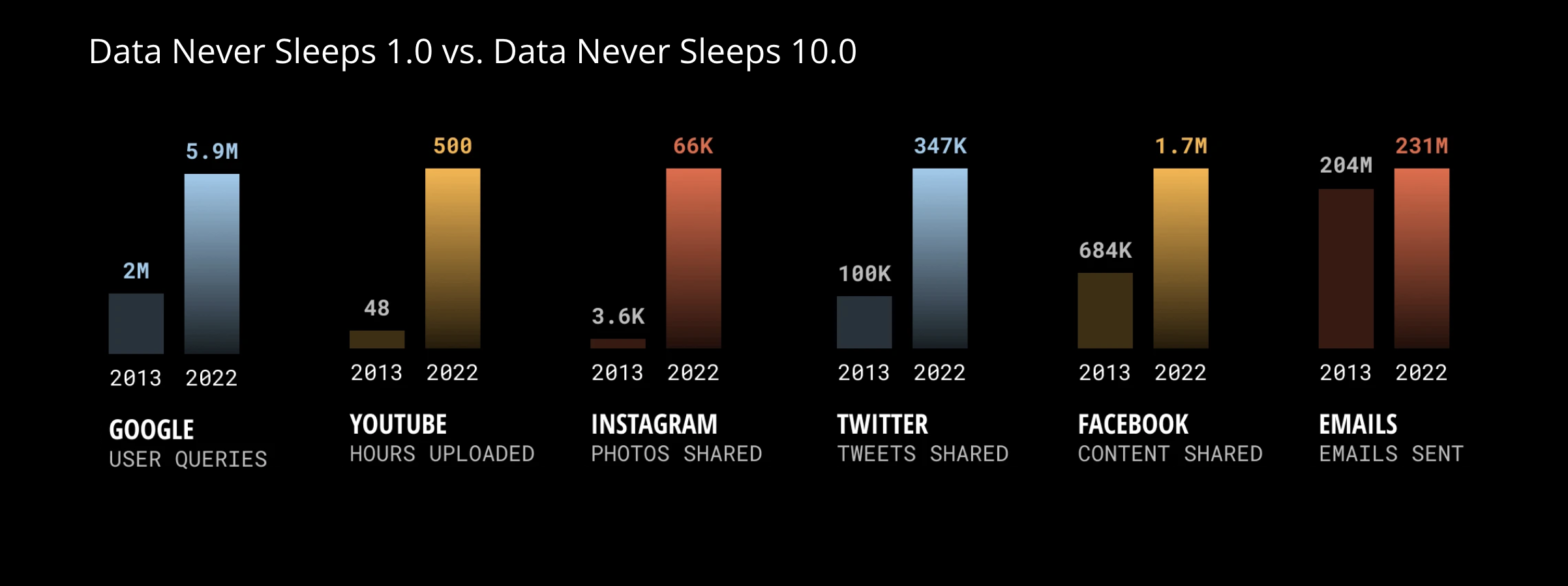
While the underlying concept is not new, the computational tools we use are relatively new. And we have a lot more data!
2.2 Data science workflow
The folks who wrote R for Data Science proposed the following data science workflow:
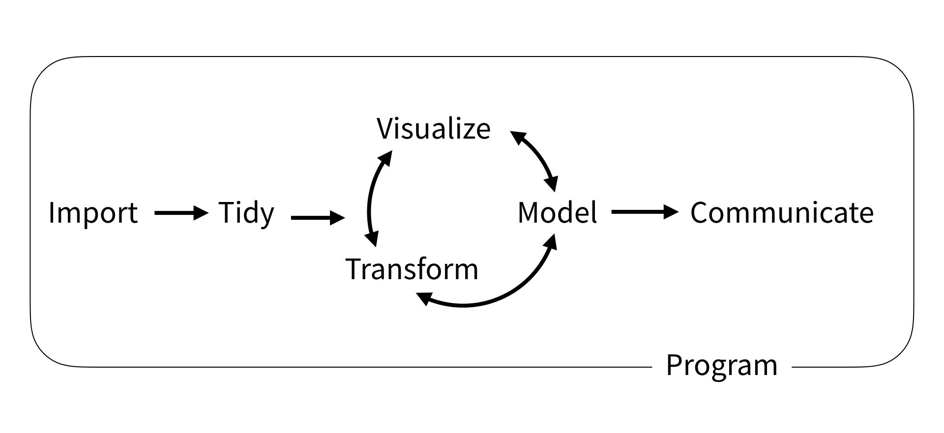
Let’s unpack what these mean briefly:
Import: gather data from a variety of sources, which can include structured data (like databases and spreadsheets) and unstructured data (like text, images, and videos).
Tidy and Transform: The raw data we import is often messy. Data scientists clean and preprocess the data, which involves removing errors, handling missing values, and transforming data into a suitable format for analysis.
Visualize (exploratory data analysis) visualize and summarize data to identify patterns, form hypotheses, select appropriate models, and guide further analysis.
Model: Using statistical methods, machine learning algorithms, and other computational techniques, data scientists build models to understand underlying patterns in the data. Models are tested using validation techniques to ensure their accuracy and reliability. Then data scientists use them to draw meaningful conclusions, like predictions about the future or inferences about populuation.
Communicate: Finally, a crucial part of data science is communicating findings clearly and effectively, whatever your purpose (academic, industry, or the public!)
Program: Surrounding all these is programming, since the computational tools are what make these possible!
Data science has applications in many fields far beyond language and the mind. It allows us to make data-driven decisions, solve complex problems, and uncover hidden insights that might not be apparent through other methods.
2.3 Overview of the course
We will spend the first few weeks getting comfortable programming in R, including some useful skills for data science:
- R basics
- Data visualization
- Data wrangling
Then, we will spend the next several weeks building a foundation in basic statistics and model building:
- Sampling distribution
- Hypothesis testing
- Model specification
- Model fitting
- Model accuracy
- Model reliability
Finally we will cover a selection of more advanced topics that are often applied in language and mind fields, with a focus on basic understanding:
- Classification
- Inference for regression
- Mixed-effect models
2.4 Syllabus, briefly
Each week will include two lectures and a lab:
- Lectures are on Tuesdays and Thursdays at 12pm and will be a mix of conceptual overviews and R tutorials. It is a good idea to bring your laptop so you can follow along and try stuff in R!
- Labs are on Thursday or Friday and will consist of (ungraded) practice problems and concept review with TAs. You may attend any lab section that works for your schedule.
There are 8 graded assessments:
- 6 Problem sets (40%) in which you will be asked to apply your newly aquired R programming skills.
- 2 Midterm exams (60%) in which you will be tested on your understanding of lecture concepts.
There are a few policies to take note of:
- Missed exams cannot be made up except in cases of genuine conflict or emergency (documentation and course action notice required). You may take the optional final exam to replace a missed or low scoring exam.
- You may request an extension on any problem set of up to 3 days. But extensions beyond 3 days will not be granted (because delying solutions will negative impact other students).
- You may submit any missed quiz or problem set by the end of the semester for half-credit (50%), even after solutions are posted.
- We will drop your lowest pset grade, but you must turn in all 6 assignements to be eligible.
2.5 Why R?
With many programming languages available for data science (e.g. R, Python, Julia, MATLAB), why use R?
- Built for stats, specifically
- Makes nice visualizations
- Lots of people are doing it, especially in academia
- Easier for beginners to understand
- Free and open source (though so are Python and Julia, MATLAB costs $)
If you are interested, here is a math professor’s take on the differences between Python, Julia, and MATLAB. Note that although they’re optimized for different things, they are all great and the technical skills and conceptual knowledge you gain in this course will transfer to other languages.
3 Google Colab
There are many ways to program with R. Some popular options include:
- R Studio
- Jupyter
- VS Code
- and even simply the command line/terminal
Google Colab is a cloud-based Jupyter notebook that allows you to write, execute, and share code like a google doc. We use Google Colab because it’s simple and accessible to everyone. You can start programming right away, no setup required! Google Colab officially supports Python and R (and secretly Julia, too!)
New R notebook:
- colab (r kernel) - use this link to start a new R notebook
File > New notebookand thenRuntime>Change runtime typeto R
Cell types:
+ Code- write and execute code+ Text- write text blocks in markdown
Left sidebar:
Table of contents- outline from text headingsFind and replace- find and/or replaceFiles- upload files to cloud session
Frequently used menu options:
File > Locate in Drive- where in your Google Drive?File > Save- savesFile > Revision history- history of changes you madeFile > Download > Download .ipynb- used to submit assignments!File > Print- printsRuntime > Run all- run all cellsRuntime > Run before- run all cells before current active cellRuntime > Restart and run all- restart runtime, then run all
Frequently used keyboard shortcuts:
Cmd/Ctrl+S- saveCmd/Ctrl+Enter- run focused cellCmd/Ctrl+Shift+A- select all cellsCmd/Ctrl+/- comment/uncomment selectionCmd/Ctrl+]- increase indentCmd/Ctrl+[- decrease indent
4 R Basics
4.1 Basics
We begin by defining some basic concepts:
- Expressions are combinations of values, variables, operators, and functions that can be evaluated to produce a result. Expressions can be as simple as a single value or more complex involving calculations, comparisons, and function calls. They are the fundamental building blocks of programming.
10- a simple value expression that evaluates to10.x <- 10- an expression that assigns the value of10tox.x + 10- an expression that adds the value ofxto10.a <- x + 10- an expression that adds the value ofxto10and assigns the result to the variablea
- Objects allow us to store various types of data, such as numbers, text, vectors, matrices; and more complex structures like functions and data frames. Objects are created by assigning values to variable names with the assignment operator,
<-. For example, inx <- 10,xis an object assigned to the value 10. - Names that we assign to objects must include only letters, numbers,
., or_. Names must start with a letter (or.if not followed by a number). - Attributes allow you to attach arbitrary metadata to an object. For example, adding a
dim(dimension) attribute to a vector allows it to behave like a matrix or n dimensional array. - Functions (or commands) are reusable pieces of code that take some input, preform some task or computation, and return an output. Many functions are built-in to base R (see below!), others can be part of packages or even defined by you. Functions are objects!
- Environment is the collection of all the objects (functions, variables etc.) we defined in the current R session.
- Packages are collections of functions, data, and documentation bundled together in R. They enhance R’s capabilities by introducing new functions and specialized data structures. Packages need to be installed and loaded before you can use their functions or data.
- Comments are notes you leave to yourself (within code blocks in colab) to document your code; comments are not evaluated.
- Messages are notes R leaves for you, after you run your code. Messages can be simply for-your-information, warnings that something unexpected might happen, or erros if R cannot evaluate your code.
Ways to get help when coding in R:
- Read package docs - packages usually come with extensive documentation and examples. Reading the docs is one of the best ways to figure things out. Here is an example from the dplyr package.
- Read error messages - read any error messages you receive while coding — they give clues about what is going wrong!
- Ask R - Use R’s built-in functions to get help as you code
- Ask on Ed - ask questions on our class discussion board!
- Ask Google or Stack Overflow - It is a normal and important skill (not cheating) to google things while coding and learning to code! Use keywords and package names to ensure your solutions are course-relevant.
- Ask ChatGPT - You can similarly use ChatGPT or other LLMs as a resource. But keep in mind they may provide a solution that is wrong or not relevant to what we are learning in this course.
4.2 Important functions
For objects:
str(x)- returns summary of object’s structuretypeof(x)- returns object’s data typelength(x)- returns object’s lengthattributes(x)- returns list of object’s attributesx- returns object xprint(x)- prints object x
For environment:
ls()- list all variables in environmentrm(x)- remove x variable from environmentrm(list = ls())- remove all variables from environment
For packages:
install.packages()to install packageslibrary()to load the package into your current R session.data()to load data from package into environmentsessionInfo()- version information for current R session and packages
For help:
?mean- get help with a functionhelp('mean')- search help files for word or phrasehelp(package='tidyverse')- find help for a package
4.3 Vectors
One of the must fundamental data structures in R is the vector. There are two types:
- atomic vector - elements of the same data type
- list - elements refer to any object (even complex objects or other lists)
Atomic vectors can be one of six data types:
double- real numbers, written in decimal (0.1234) or scientific notation (1.23e4)- numbers are double by default (3 is stored as 3.00)
- three special doubles:
Inf,-Inf, andNaN(not a number)
integer- integers, whole numbers followed byL(3L or 1e3L)character- strings with single or double quotes (‘hello world!’ or “hello world!”)logical- boolean, written (TRUEorFALSE) or abbreviated (TorF)complex- complex numbers, whereiis the imaginary number (5 + 3i)raw- stores raw bytes
To create atomic vectors:
c(2,4,6)-c()function for combining elements, returns2 4 62:4-:notation to construct a sequence of integers, returns2 3 4seq(from = 2, to = 6, by=2)-seq()function to create an evenly-spaced sequence, returns2 4 6
To check an object’s data type:
typeof(x)- returns the data type of object xis.*(x)- test if object x is data type, returnsTRUEorFALSEis.double()is.integer()is.character()is.logical()
To change an object to data type (explicit coercion):
as.*(x)- coerce object to data typeas.double()as.integer()as.character()as.logical()
Note that atomic vectors must contain only elements of the same type. If you try to include elements of different types, R will coerce them into the same type with no warning (implicit coercion) according to the heirarchy character > double > integer > logical.
4.4 Operations
Arithmetic operators:
+- add-- subtract*- multiply/- divide^- exponent
Comparison operators return true or false:
a == b- equal toa != b- not equal toa > b- greater thana < b- less thana >= b- greater than or equal toa <= b- less than or equal to
Logical operators combine multiple true or false statements:
&- and|- or!- notany()- returns true if any element meets conditionall()- returns true if all elements meet condition%in%- returns true if any element is in the following vector
Most math operations (and many functions) are vectorized in R:
- they can work on entire vectors, without the need for explicit loops or iteration.
- this a powerful feature that allows you to write cleaner, more efficient code
- To illustrate, suppose
x <- c(1, 2, 3):x + 100returnsc(101, 102, 103)x == 1returnsc(TRUE, FALSE, FALSE)
4.5 More complex structures
Some more complex data structures are built from atomic vectors by adding attributes:
matrix- a vector with adimattribute representing 2 dimensionsarray- a vector with adimattribute representing n dimensionsfactor- an integer vector with two attributes:class="factor"andlevels, which defines the set of allowed values (useful for categorical data)date-time- a double vector where the value is the number of seconds since Jan 01, 1970 and atzoneattribute representing the time zonedata.frame- a named list of vectors (of equal length) with attributes fornames(column names),row.names, andclass="data.frame"(used to represent datasets)
To create more complex structures:
list(x=c(1,2,3), y=c('a','b'))- create a listmatrix(x, nrow=2, ncol=2)- create a matrix from a vectorxwith nrow and ncolarray(x, dim=c(2,3,2))- create an array from a vectorxwith dimensionsfactor(x, levels=unique(x))- turn a vectorxinto a factordata.frame(x=c(1,2,3), y=c('a','b','c'))- create a data frame
Missing elements and empty vectors:
NA- used to represent missing or unknown elements in vectors. Note thatNAis contageous: expressions includingNAusually returnNA. Check forNAvalues withis.na().NULL- used to represent an empty or absent vector of arbitrary type.NULLis its own special type and always has length zero andNULLattributes. Check forNULLvalues withis.null().
4.6 Subsetting
Subsetting is a natural complement to str(). While str() shows you all the pieces of any object (its structure), subsetting allows you to pull out the pieces that you’re interested in. ~ Hadley Wickham, Advanced R
There are three operators for subsetting objects:
[- subsets (one or more) elements[[and$- extracts a single element
There are six ways to subset multiple elements from vectors with [:
x[c(1,2)]- positive integers select elements at specified indexesx[-c(1,2)]- negative integers select all but elements at specified indexesx[c("name", "name2")]select elements by name, if elements are namedx[]- nothing returns the original objectx[0]- zero returns a zero-length vectorx[c(TRUE, TRUE)]- select elements where corresponding logical value isTRUE
These also apply when selecting multiple elements from higher dimensional objects (matrix, array, data frame), but note that:
- indexes for different dimensions are separated by commas
[rows, columns, ...] - omitted dimensions return all values along that dimension
- the result is simplified to the lowest possible dimensions by default
- data frames can also be indexed like a vector (selects columns)
There are 3 ways to extract a single element from any data structure:
[[2]]- a single positive integer (index)[['name']]- a single stringx$name- the$operator is a useful shorthand for[['name']]
When extracting single elements, note that:
[[is preferred for atomic vectors for clarity (though[also works)$does partial matching without warning; useoptions(warnPartialMatchDollar=TRUE)- the behavior for invalid indexes is inconsistent: sometimes you’ll get an error message, and sometimes it will return
NULL
4.7 Built-in functions
Note that you do not need to memorize these built-in functions to be successful on quizzes. Use this as a reference.
For basic math:
log(x)- natural logexp(x)- exponentialsqrt(x)- square rootabs(x)- absolute valuemax(x)- largest elementmin(x)- smallest elementround(x, n)- round to n decimal placessignif(x, n)- round to n significant figuressum(x)- add all elements
For stats:
mean(x)- meanmedian(x)- mediansd(x)- standard deviationvar(x)- variancequantile(x)- percentage quantilesrank(x)- rank of elementscor(x, y)- correlationlm(x ~ y, data=df)- fit a linear modelglm(x ~ y, data=df)- fit a generalized linear modelsummary(x)- get more detailed information from a fitted modelaov(x)- analysis of variance
For vectors:
sort(x)- return sorted vectortable(x)- see counts of values in a vectorrev(x)- return reversed vectorunique(x)- return unique values in a vectorarray(x, dim)- transform vector into n-dimensional array
For matrices:
t(m)- transpose matrixm %+% n- matrix multiplicationsolve(m, n)- find x in m * x = n
For data frames:
view(df)- see the full data framehead(df)- see the first 6 rows of data framenrow(df)- number of rows in a data framencol(df)- number of columns in a data framedim(df)- number of rows and columns in a data framecbind(df1, df2)- bind dataframe columnsrbind(df1, df2)- bind dataframe rows
For strings:
paste(x, y, sep=' ')- join vectors together element-wisetoupper(x)- convert to uppercasetolower(x)- convert to lowercasenchar(x)- number of characters in a string
For simple plotting:
plot(x)values of x in orderplot(x, y)- values of x against yhist(x)- histogram of x
4.8 Programming in R
Writing functions and handling control flow are important aspects of learning to program in any language. For our purposes, some general conceptual knowledge on these topics is sufficient (see below). Those interested to learn more might enjoy the book Hands-On Programming with R.
Functions are reusable pieces of code that take some input, perform some task or computation, and return an output.
function(inputs){
    ## do something
    return(output)
}
Control flow refers to managing the order in which expressions are executed in a program:
if…else- if something is true, do this; otherwise do thatforloops - repeat code a specific number of timeswhileloops - repeat code as long as certain conditions are truebreak- exit a loop earlynext- skip to next iteration in a loop
5 Further reading and references
Suggested further reading:
- Getting started with Data in R from Modern Dive textbook
- R Nuts and Bolts in R Programming for Data Science by Roger Peng
- Base R Cheat Sheet
Other references:
- Vectors in Advanced R by Hadley Wickham
- Subsetting in Advanced R by Hadley Wickham
- A field guide to base R in R for Data Science by Hadley Wickham